Myriad Trainer

Introduction

The Myriad Model Trainer is a desktop application designed to ease the process of training machine learning models for Region Of Interest (ROI) detection applications. The trainer is not required; Myriad the library and applications written using the library will run without its usage.

The basic workflow behind Myriad Trainer is as follows.

1. Gather training data representative of the ROI, including both positive (i.e. known to contain the ROI) and negative (i.e. known to not contain the ROI) samples.
2. Feed the training data to a prospective model to train it to detect ROI.
3. If the model is promising, save its current state for use in Myriad.
4. (Optional) Return to Step 1.

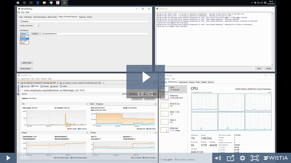
A video demonstrating the basic usage of Trainer and its companion tool Desktop is also available:

Installation

The Myriad library must be installed prior to building Trainer. Please refer to the main Installation page for details on installing Myriad, Myriad Trainer, and Myriad Desktop.

Inital Preparation

Acquiring Data

The training data should be representative of the types of ROI the model will ultimately be used to detect. The specificity of the data will depend on the application and the user’s goals for the model. When used to detect indications of structural damage in nondestructive evaluation (NDE) data for example a user may wish to train a model for looking at C-scans and another for A-scans, or one model for pitting and another for cracks, etc.

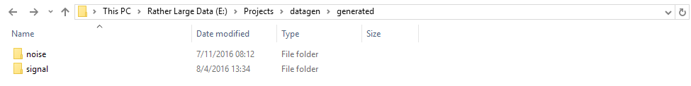
The training data should be organized into two categories. Positive samples (referred to as “signal” in Myriad Trainer) should be stored in one folder, and negative samples (“noise”) in another. The trainer expects that all of the samples in a given folder are of the same category. Each file should consist of a single sample, and can be of any format supported by Myriad. The files do not all have to be of the same format, e.g. CSV and bitmap images can co-exist in the same folder.

Regardless of file type or size, each sample in the training set must have the same number of elements. When a machine learning model is trained, each sample’s elements are considered “features” to be learned, e.g. if all the samples are 15x15 elements the feature vector has 225 features. If one or more samples vary in their number of elements the model would consider the smaller samples to be missing features. If samples within the training data set vary in their number of elements, consider padding with 0’s or resizing as required.

Once a model has been built to expect a specific number of features, that model can only be trained with or make predictions on samples that are the same size. Careful consideration should be given to the number of features when building a model. As a consequence of the “curse of dimensionality” in machine learning, the more features that are used the more data are generally required to train a useful model. At the same time however smaller feature vectors directly corresponds to smaller regions, which can be computationally expensive for very large datasets.

One recommended approach is to use the “natural” size of the ROI as a guide. If the typical ROI for the current application occupies a box of 50x100 elements for example, consider using samples that are 50x100. The Myriad library provides scale-invariance for machine learning so the only requirement when using the final model is to use this same 50x100 box during the “sliding window” phase of data processing to ensure that the model receives the expected feature vector.

Generally speaking, the more data available for training the better. Frequently in ROI detection the number of negative samples greatly exceeds the number of positive samples. This can be partially addressed through generating “artificial” positive samples by e.g. rotating the available positive samples by 90, 180, and 270 degrees and adding Gaussian noise. Myriad Trainer also provides an option for attempting to balance the ratio between positive and negative samples if preferred. Since Myriad’s machine learning models are incremental or “online” learners, it’s worth remembering that a model can be trained at any time - even after it’s being used. Thus a model’s incorrect calls can be turned into training data to improve its future performance.

Sample folders are added to the available data by pressing the + button and typing or browsing to the folder in question. Before accepting the new folder be certain to set the type of samples within the folder: positive samples should be set to signal and negative samples to noise. Click OK to add the folder to the available data.

Example - Ultrasonic Data

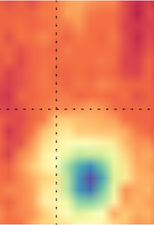
As an example of the general approach to compiling a training data set, consider Myriad's original application - detecting indications of structural damage in sensor data. A frequently-encountered data presentation for structural inspections is the C-scan in which the damage sensor is rastered above the part to be inspected. Here's an example of an ultrasonic sensor C-scan of a structure with a defect in the corner:

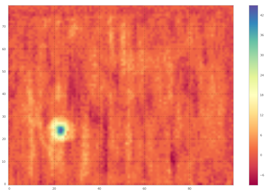
Although we could use this entire slice as a single sample, there are two main drawbacks to this approach.

1. We'd only have 1 sample.
2. The sample is fairly large, so model training time, data processing, etc. will take longer.

An alternative approach is to consider smaller pieces of this scan:

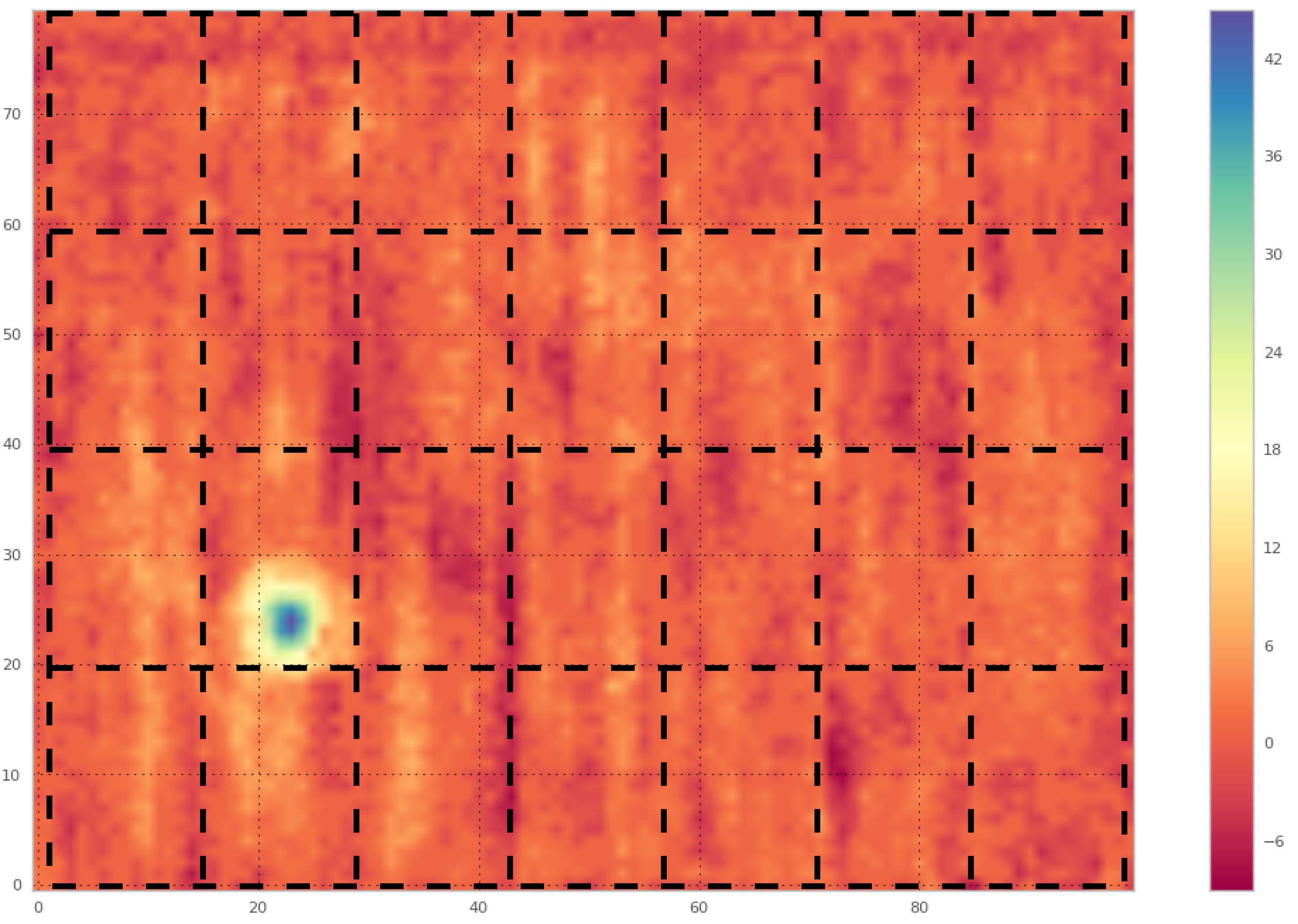
If we export each of these regions as a separate sample, we would now have 28 samples rather than the original 1. In this case, we will have 27 "noise" (i.e. don't contain a flaw signal) samples that will look something like this:

And 1 "signal" (i.e. does contain a flaw signal) sample:

How the data subset extraction and export is performed will vary depending on the input format and the tools available; for images the most straightforward approach is to simply open the image in an image editor and manually extract the regions. If you're comfortable with Java, Myriad's Sliding Window operation can be used to do this extraction automatically - just examine the results and organize into signal and noise folders:

If we've captured the complete ultrasonic waveform, we can then repeat this process for each "slice" of the three-dimensional data. If we're working off of a single exported slice, we will need to acquire more data before we can proceed with training.

Preprocessing Sample Data

In many ROI applications, relying on signal amplitude alone will not produce useful models. Applying one or more preprocessing operations to the data can make implicit features in the data explicit, which in turn makes a machine learning model more accurate. In building machine learning models that parse log files for example, it is common to take timestamps that record elapsed seconds since 1970 such as 1473085969 and convert it into an explicit month, day, year, and time. In effect, this simple operation turns one field into four and might help the model recognize that e.g. logins over the weekend are unusual.

In image processing and object detection applications some of the most-frequently used forms of preprocessing involve normalization and convolution operations such as Sobel edge detection or the Histogram of Oriented Gradients (HOG) algorithm. Several such operations are available within Myriad Trainer and can be applied to data before it is sent to a prospective model. For ROI detection, Canny edge detection is a good place to start - it tends to produce better edges than Sobel or other simpler edge detection algorithms. At the same time, it is computationally cheaper than HOG; an important consideration as the preprocessing operation chosen here must be performed when the model is deployed and used to examine “real” data.

Alternatively, preprocessing can be applied to the sample data before it is loaded in Myriad Trainer if desired. External data processing applications such as Mathematica, Matlab or Python can be used to read each sample file and apply the desired preprocessing. Note that as mentioned above any preprocessing done during training must also be performed when using the trained model. Generally speaking it isn’t sufficient to use the same algorithm from different platforms (e.g. training with Matlab’s HOG and using Myriad’s HOG) because implementations can differ.

Emphysic recommends that when using external preprocessing that this preprocessing becomes part of your ROI detection code whenever possible, i.e. your code expects to receive “undoctored” data and applies its own preprocessing as required. This ensures that your ROI detector always gets the correct inputs and makes it more portable.

Train / Test Data

Frequently when training a machine learning model it is common to set aside some subset of the training data, and training a model on the remainder. The subset left out of training can then be used to test the model’s performance. By default Myriad Trainer leaves 20-25% of the training data aside for testing, using 75-80% for training. This can be adjusted as desired, although the program will not allow the percentage of data used for training or for testing to be less than 1%.

To build the training and test data sets, Myriad Trainer randomly selects samples until the percentages are met.

Training Considerations

Overfitting

It can be tempting to reduce the test data percentage down and watch the accuracy of the model improve. It’s important to remember however that this can easily result in “overfitting” the model to your training data, a condition in which the model learns too much about the characteristics of your training data and is then unable to make general predictions. This condition is most easily observed if a model achieves very high accuracies during training and then performs poorly in “real world” tests. The model has effectively memorized the test but not the lesson. By keeping some small percentage of training data away from the model, its evaluation is performed on data it has never encountered and is a more realistic evaluation metric.

Label Balancing

By default the trainer will attempt to balance the number of positive and negative samples in a training set so that the ratio of positive:negative samples is approximately 1. If your training data is extremely unbalanced (e.g. number of negative samples >> number of positive samples), this can reduce the amount of data available for training. At the same time however disabling this balancing can have a detrimental effect on the model - if the ratio is 100:1 for example the model could simply learn to always predict the more frequent category and still show an impressive accuracy.

Since the models are incremental learning algorithms, an alternative to disabling balancing is simply to start using the model in the “real world.” When a model makes an incorrect prediction, the data can be added to a new training set. The model is opened in Myriad Trainer and trained on the new results, saved, deployed, and the process repeated.

Running Experiments

Emphysic recommends planning a basic design of experiments prior to beginning the model training and evaluation process. For each preprocessing or model configuration option, the subsequent model should be saved with a meaningful name. After an initial round of evaluation has completed, the most promising model can be developed further. Several open source tools are available that can generate the parameters for your study, including:

• GNU Octave's fullfact() function
• Python's pyDOE package
• Scilab's Design of Experiments Toolbox
• javamut

Choosing An Algorithm

Myriad uses Smile and Apache Mahout for its machine learning functionality. As of this writing the following algorithms are directly available in Myriad.

1. Stochastic Gradient Descent (SGD) - also known as steepest descent. A stochastic approximation to gradient descent, in which the direction of the local gradient is found and steps are taken in the negative of this direction.
2. Adaptive Stochastic Gradient Descent (ASGD) - an “ensemble” learning method in which multiple SGD models are trained and the “best” are used for predictions.
3. Passive Aggressive (PA) - for a weight vector W initialized with 0 in each element, calculate the loss at each step L = max(0, 1 - yd_TW) where y is the actual category of the sample d and d_T is the transpose of d. Update the weight vector as Wnew = w + yLd and repeat.
4. Gradient Machine - a gradient machine learner with one hidden sigmoid layer that attempts to minimize hinge loss. Currently in development and should be considered experimental.

Each algorithm has its strengths and weaknesses; Emphysic recommends that each be evaluated during an initial experiment. Note that for SGD in particular it is possible that Myriad Trainer will report that no useful results were returned; this is an indication that the model was unable to learn any difference between the positive and negative samples. If you are using a train and a test set, additional attempts may address the issue.

Training

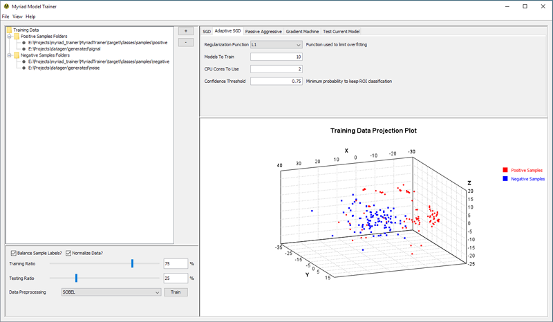
To create a new model, select an algorithm to use by choosing the appropriate tab in the Myriad Trainer interface e.g. create a new Passive Aggressive model by making the Passive Aggressive tab visible. Adjust the train:test ratios, sample balancing, and preprocessing operations (if any) as desired.

Trainer also provides an option for automatically normalizing the samples such that each value in each sample is scaled to lie between 0 and 1. If a machine learning algorithm is sensitive to feature scaling (as is the case with SGD algorithms), normalizing the data can improve the model's performance. As with preprocessing operations in general, we recommend conducting experiments with your data to determine whether accuracies improve with normalization.

When the Train button is pressed, Myriad Trainer will attempt to read each of the folders specified. For each file in each of the folders, the trainer will attempt to load the contents as a Myriad dataset and if successful will assign the appropriate label to the dataset. When all the available data have been read, a random subset is set aside for testing and the remainder used to train the selected model. At the same time, the trainer will produce a plot that visualizes a projection of the entire dataset in three dimensions, with red markers indicating positive samples and blue indicating negative. The projection is based on Principal Component Analysis.

For each sample in the training set, the model is sent a one-dimensional array of the sample’s data and a label indicating whether the sample is positive or negative. After the training is complete, Myriad Trainer tests the model’s accuracy by asking it to predict the category of each sample in the testing set. By default, Trainer will repeat this process 100 times to generate an average accuracy (% of correct calls) for the model.

If a model exists in memory and the Train button is pressed Myriad Trainer will ask whether the current model should undergo another round of training. If replacement is chosen, the previous model is scrapped and a new model is created. A model can be trained in as many or as few rounds of training as desired. During each round of training it is important that the same preprocessing and model configuration parameters are used.

To load a previously-saved model, select Open Model and browse to the folder chosen when the model was saved. If a model was in system memory, it is replaced with the model read from disk and its accuracy set to 0.

Testing

To evaluate a model’s performance after a round of training, switch to the Test Current Model tab. By default Myriad Trainer will randomly select 100 points for testing, but this number can be adjusted as desired.

When the Run Test button is pressed Myriad Trainer selects the specified number of test samples from the available data, reads and applies any preprocessing, and then has the current model predict their labels. When complete the accuracy of the model is reported, and the trainer plot visualizes the results by plotting the test data. Red points are those points that are known to be positive samples and blue are points known to be negative samples. Correctly-predicted points are drawn with circles, and incorrect are drawn with X’s. As such there are four possible categories shown in the visualization:

1. Samples that are positive and were predicted positive are red circles.
2. Samples that are positive but were predicted negative are red X’s.
3. Samples that are negative and were predicted negative are blue circles.
4. Samples that are negative and were predicted positive are blue X’s.

If one or more categories are not seen in the visualization, no samples were found in that category. A 100% accurate model would therefore only have two types of points: red and blue circles indicating the correctly-labelled positive and negative samples respectively.

As a rule of thumb for assessing a model, a model performs better than random guessing if its accuracy is greater than 50%. The higher the accuracy the better, although when accuracy exceeds 90% it may be an indication of overfitting.

Improving Model Performance

Low Accuracy During Test/Train Cycle

When presented with a model that does not perform as accurately as desired, several steps can be taken. Several options are discussed in this section, roughly ordered from least to most drastic.

Contact Emphysic

As a first step if you run into any difficulties creating useful models or using any of the Myriad tools, consider contacting Emphysic. We wrote it, we use it, and we may be able to provide a few ideas to save you some work.

Get More Data

In general the more data the model can learn from the better. If possible, acquire more data to be used during the training process. If none are available, consider means of “artificially” generating new data. One option discussed previously: for each sample in the training data, rotate through 90, 180, and 270 degrees so that one “real” sample is actually represented four times. By applying an operation such as adding random noise or a blur to each of these four samples, a dataset can be greatly expanded.

Adjust Confidence Threshold

Several of the machine learning algorithms available in Trainer calculate the probabilities of a sample containing ROI. These algorithms have a “confidence threshold” that can be adjusted to make the model more or less conservative in its classifications.

By default the threshold is set to 0.75, meaning that the model must assign a probability of 75% or more to a sample to label it as ROI. If the model’s probability is below this threshold, samples labelled ROI are re-labelled as not containing ROI.

If a model appears to be making too many false ROI calls, try adjusting the confidence threshold higher. When set to 1, the model must be 100% confident the sample is ROI for it to be labelled as such. Conversely if a model appears to be missing ROI, try adjust the threshold lower. When set to 0 confidence thresholds are disabled so that all ROI are called as such regardless of probability.

Incremental Training

Consider putting the model into service and saving the data. In particular, a procedure known as hard negative mining takes the data that were incorrectly labelled as positive samples and uses them in the next round of training for the model. In some applications a model can learn to distinguish positive and negative samples on the periphery but may have trouble differentiating closer to the decision boundary (the region where labels are ambiguous). Hard negative mining can help improve the accuracy of a model not just by correctly labelling mis-labelled samples but also by helping to more narrowly define the decision boundary.

Preprocessing

Myriad has multiple preprocessing operations that can be applied to training data. As mentioned previously, edge detection algorithms including Sobel, Scharr, Prewitt, and Canny can often make implicit features in data explicit. Canny edge detection in particular is a good place to start because it has the side effect of normalizing the data between 0 and 1, which can help to remove variations in amplitude that might otherwise confuse an ROI detector.

Normalizing can also be performed in combination with other preprocessing operations by enabling the Normalize Data? checkbox and selecting the preprocessing operation of choice. The data will be normalized prior to performing the preprocessing operation.

If edge / blob detection algorithms do not improve results, a more elaborate algorithm such as Histogram of Oriented Gradients (HOG) is worth considering. The HOG algorithm was written specifically to encode details of gradients or edge directions in ROI detection. Although it is a more computationally expensive operation than edge detection, it may ultimately provide better results.

Change Algorithm Parameters

Some algorithms present one or more options for changing their behavior, from the penalty they incur for a wrong answer to the maximum number of iterations in their training. Although a thorough examination of each algorithm is beyond the scope of this document, a good starting point is to change a single parameter and evaluate its effect on the resultant model’s accuracy. Keeping good records of configurations investigated and their results are crucial.

Change Algorithm

Several machine learning algorithms are available in Myriad, and it is worth considering each when an initial model does not meet expectations. Each has its own strengths and weaknesses, and depending upon the nature of your application you may find one algorithm performs better than another.

Switch Tools

Myriad Trainer provides a starting point for machine learning model development, but it is not intended to function as a complete ML development environment. For a more detailed data science project it may be worthwhile to use an external toolset to conduct your initial investigations and then move back to Myriad when you achieve promising results.

Many technical computing platforms offer data science and machine learning capabilities. Some of these platforms include:

• Matlab’s Statistics and Machine Learning Toolbox (Commercial)
• Mathematica 10+ (Commercial)
• Python and the scikit-learn package
  • A prepackaged version of Python and an extensive toolset for data science is available from Continuum
• Weka desktop analytics tool